1. Installation
1.1. Requirements
Installation of celmech will require a few additional Python packages.
1.2. GitHub
In order to install celmech you will first need to clone the GitHub
repository located here. This can be
accomplished from the terminal by first navigating to the desired target
directory and then issuing the command:
git clone https://github.com/shadden/celmech.git
After you have cloned the git repository, navigate into the top celmech directory and issue the terminal command:
python setup.py install
in order to install the Python package.
1.3. Pip
celmech is available through PyPI and can be
installed with the terminal command:
pip install celmech
2. A First Example
Now that celmech is installed, we’ll run through a short example of how to
use it. In our example we’ll use it in conjunction with the rebound N-body
integrator to build and integrate a simple Hamiltonian model for the dynamics
of a pair of planets in a mean motion resonance. The example presented below
is also available as a Jupyter notebook on GitHub.
2.1. Setup
We’ll start by importing the requisite packages.
import numpy as np
import rebound as rb
from celmech import Poincare, PoincareHamiltonian
from sympy import init_printing
init_printing() # This will typeset symbolic expressions in LaTeX
Now we’ll initialize a rebound simulation containing a pair of Earth-mass
planets orbiting a central solar-mass star with a 3:2 period ratio
commensurability.
sim = rb.Simulation()
sim.add(m=1,hash='star')
sim.add(m=3e-6,P = 1, e = 0.03,l=0)
sim.add(m=3e-6,P = 3/2, e = 0.03,l=np.pi/5,pomega = np.pi)
sim.move_to_com()
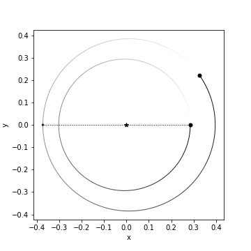
rb.OrbitPlot(sim,periastron=True)
After running the above code, we should see a represntation of our planetary system:
We’d like a construct a Hamiltonian that can capture the dynamical evolution of
the system. To start, we’ll initialize a Poincare
object in order to represent our system and a
PoincareHamiltonian object to model its dynamical
evolution. These objects can be initialized directly from the rebound
simulation that we created above:
pvars = Poincare.from_Simulation(sim)
pham = PoincareHamiltonian(pvars)
Now that we’ve now generated a PoincareHamiltonian
object, we’ll examine the symbolic expression for the Hamiltonian governing our
system:
pham.H
which should display:
This expression is the just Hamiltonian of two non-interacting Keplerian orbits
expressed in canonical variables used by celmech. The canonical momenta
for the \(i\)-th planet are defined [1] in terms of the planet’s standard
orbital elements
\((a_i,e_i,I_i,\lambda_i,\varpi_i,\Omega_i)\) and mass parameters
\(\mu_i\sim m_i\) and \(M_i \sim M_*\):
and their conjugate coordinates are:
When a PoincareHamiltonian is first initialized, it
will only contain the ‘Keplerian’ terms of the Hamiltonian and will not contain
any terms representing gravitaional interactions between the planets. This
will result in quite boring dynamical evolution: the planets’ mean longitudes,
\(\lambda_i\), will simply increase linearly with time at a rate of
\(n_i = \frac{G^{2} M_{2}^{2} m_{i}^{3}}{\Lambda_{i}^{3}}\), while all
other orbital elements remain constant.
In order explore more interesting dynamics, we need to add terms to Hamiltonian that capture pieces of the gravitational interactions between planets. Since our planet pair is near a 3:2 MMR, terms associated with this resonance are a natural choice to explore. For a pair of co-planar planets, these terms will all involve linear combinations of the two resonant angles
In fact, at lowest order in the planets’ eccentricities, there are just two
such terms, \(\propto e_1\cos\theta_1\) and \(\propto
e_2\cos\theta_2\). The method
add_MMR_terms() provides a
convenient method for adding these terms to our Hamiltonian:
pham.add_MMR_terms(3,1,max_order=1)
pham.H
which should now display
This somewhat cumbersome expression is just equivalent to
but expressed in the canonical variables used by celmech. [2]
2.2. Integration
Now that we have a Hamiltonain model, we’ll integrate it and compare the results to direct \(N\)-body. First, we’ll set up some preliminary python dictionaries and arrays to hold the results of both integrations.
# Here we define the times at which we'll get simulation outputs
Nout = 150
times = np.linspace(0 , 3e3, Nout) * sim.particles[1].P

# These are the quantites we'll track in our rebound and celmech integrations
keys = ['l1','l2','pomega1','pomega2','e1','e2','a1','a2']

# These dictionaries will hold our results
rebound_results= {key:np.zeros(Nout) for key in keys}
celmech_results= {key:np.zeros(Nout) for key in keys}

# These are the lists of particles in both simulations
# for which we'll save quantities.
rb_particles = sim.particles
cm_particles = pvars.particles
The PoincareHamiltonian class inherits the method
integrate() that can be used to evolve
the system forward in much the same way as rebound’s
rebound.Simulation.integrate() method. Below is the main integration
loop where we’ll integrate our system and store the results:
for i,t in enumerate(times):
    sim.integrate(t) # advance N-body
    pham.integrate(t) # advance celmech
    for j,p_rb,p_cm in zip([1,2],rb_particles[1:],cm_particles[1:]):
        # store N-body results
        rebound_results["l{}".format(j)][i] = p_rb.l
        rebound_results["pomega{}".format(j)][i] = p_rb.pomega
        rebound_results["e{}".format(j)][i] = p_rb.e
        rebound_results["a{}".format(j)][i] = p_rb.a

        # store celmech results
        celmech_results["l{}".format(j)][i] = p_cm.l
        celmech_results["pomega{}".format(j)][i] = p_cm.pomega
        celmech_results["e{}".format(j)][i] = p_cm.e
        celmech_results["a{}".format(j)][i] = p_cm.a
Finally, we’ll plot the simulation results in order to compare them:
# First, we compute resonant angles for both sets of results
for d in [celmech_results,rebound_results]:
    d['theta1'] = np.mod(3 * d['l2'] - 2 * d['l1'] - d['pomega1'],2*np.pi)
    d['theta2'] = np.mod(3 * d['l2'] - 2 * d['l1'] - d['pomega2'],2*np.pi)

# Now we'll create a figure...
import matplotlib.pyplot as plt
fig,ax = plt.subplots(3,2,sharex = True,figsize = (12,8))
for i,q in enumerate(['theta','e','a']):
    for j in range(2):
        key = "{:s}{:d}".format(q,j+1)
        ax[i,j].plot(times,rebound_results[key],'k.',label='$N$-body')
        ax[i,j].plot(times,celmech_results[key],'r.',label='celmech')
        ax[i,j].set_ylabel(key,fontsize=15)
        ax[i,j].legend(loc='upper left')

#... and make it pretty
ax[0,0].set_ylim(0,2*np.pi);
ax[0,1].set_ylim(0,2*np.pi);
ax[2,0].set_xlabel(r"$t/P_1$",fontsize=15);
ax[2,1].set_xlabel(r"$t/P_1$",fontsize=15);
This should produce a figure that looks something like this:
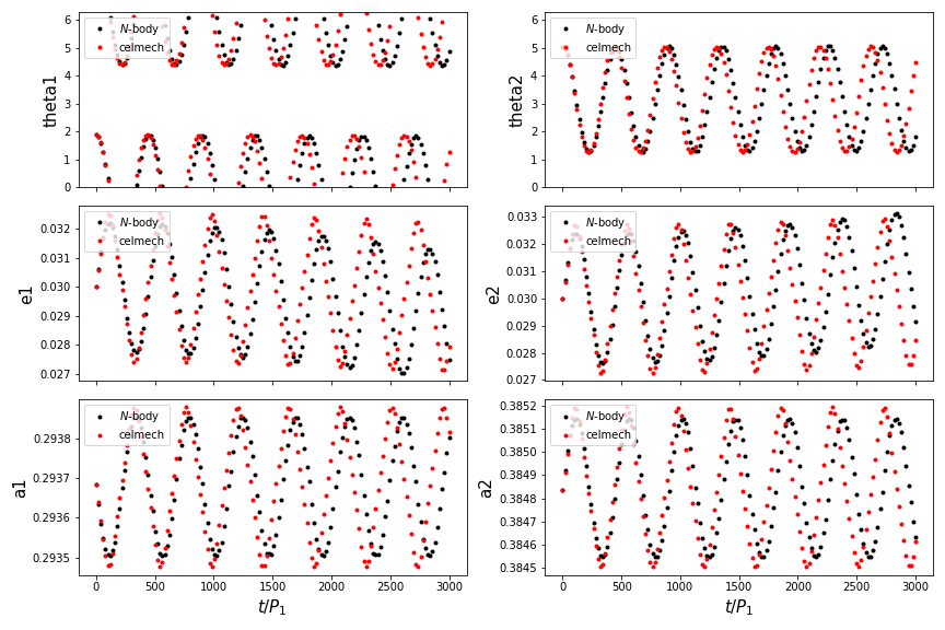
Not too bad! Our celmech model reproduces the libration amplitudes and
frequencies observed in the \(N\)-body results quite successfully.
2.3. Next steps
For a more detailed example (discussed in Sec. 2 of the paper) that incorporates additional corrections to better approximate the N-body evolution, see AddingDisturbingFunctionTerms.ipynb.
You can also check out the rest of the documentation for many other features. Another good starting point for exploration are the numerous Jupyter notebook examples available on GitHub.