6. Canonical Transformations

A transformation of canonical variables \(T:({q},{p}) \rightarrow ({q}',{p}')\) that leaves Hamilton’s equations unaltered so that

\[\begin{split}\begin{align} \frac{d}{dt}q' &= \frac{\partial}{\partial p'} H(q(q',p'),p(q',p')) \\ \frac{d}{dt}p' &= -\frac{\partial}{\partial q'} H(q(q',p'),p(q',p')) \end{align}\end{split}\]

is called a canonical transformation. Often the equations of motion encountered in celestial mechanics problems can be simplified by appropriately chosen canonical coordinate trasformations.

This documentation isn’t an introduction to canonical transformations, though there are several standard references, e.g., Goldstein’s Classical Mechanics.

6.1. The CanonicalTransformation class

The class CanonicalTransformation provides a framework for composing and applying such transformations. An instance of a CanonicalTransformation is initialized with a set of rules for transforming from old to new variables and vice versa. These rules can be applied to any expressions involving canonical variables by using the old_to_new() and new_to_old() methods. Additionally, the canonical transformation can be applied to a Hamiltonian instance in order to produce a new Hamiltonian object that has the new variables as canonical variables and with the Hamiltonian appropriately transformed.

As an example, we’ll apply a canonical transformation to simplify the toy Hamiltonian

\[H(q,p) = \frac{p_{1}^{2}}{2} + p_{2}^{4} + p_{2} + \cos{\left(3 q_{1} + 2 q_{2} \right)}\]

First, we’ll set up a Hamiltonian object to represent this system

from celmech import CanonicalTransformation, Hamiltonian, PhaseSpaceState
import sympy as sp
import numpy as np
p1,p2,q1,q2 = sp.symbols("p(1:3),q(1:3)")
H = p1**2/2 + p2 +  p2**4 + sp.cos(3*q1 + 2 * q2)
state=PhaseSpaceState([q1,q2,p1,p2],np.random.uniform(-0.5,0.5,4))
ham = Hamiltonian(H,{},state)

Next, we’ll build a canonical transformation to new variables \((Q_i,P_i)\) according to \(\mathbf{Q} = T\cdot \mathbf{q}\) and \(\mathbf{P} = (T^{-1})^\mathrm{T} \cdot \mathbf{p}\) for a matrix \(T\). We’ll construct our transformations so that \(Q_1 = 3q_1+2q_2\), the argument of the cosine term appearing in the original Hamiltonian and we’ll set \(Q_2 = q_2\).

We use the CanonicalTransformation class method from_linear_angle_transformation() to produce a CanonicalTransformation instance representing the desired transformation:

Tmtrx = [[3,2],[0,1]]
qp_old = ham.qp_vars
ct = CanonicalTransformation.from_linear_angle_transformation(qp_old,Tmtrx)

We examine the resulting transformation by expressing each old canonical variable in terms of new variables and vice versa

for variable in ct.old_qp_vars:
    exprn = ct.old_to_new(variable)
    display((variable,exprn))

for variable in ct.new_qp_vars:
    exprn = ct.new_to_old(variable)
    display((variable,exprn))

which produces the output

\[\displaystyle \left( q_{1}, \ \frac{Q_{1}}{3} - \frac{2 Q_{2}}{3}\right)\]

\[\displaystyle \left( q_{2}, \ Q_{2}\right)\]

\[\displaystyle \left( p_{1}, \ 3 P_{1}\right)\]

\[\displaystyle \left( p_{2}, \ 2 P_{1} + P_{2}\right)\]

\[\displaystyle \left( Q_{1}, \ 3 q_{1} + 2 q_{2}\right)\]

\[\displaystyle \left( Q_{2}, \ q_{2}\right)\]

\[\displaystyle \left( P_{1}, \ \frac{p_{1}}{3}\right)\]

\[\displaystyle \left( P_{2}, \ - \frac{2 p_{1}}{3} + p_{2}\right)\]

Now we’ll use our canonical transformation to generate a new Hamiltonian with the old_to_new_hamiltonian() method:

kam = ct.old_to_new_hamiltonian(ham,do_reduction=True)
kam.H

The final line displays the transformed Hamiltonian in terms of the new variables:

\[\displaystyle \frac{9 P_{1}^{2}}{2} + 2 P_{1} + P_{2} + \left(2 P_{1} + P_{2}\right)^{4} + \cos{\left(Q_{1} \right)}\]

After the transformation, the Hamiltonian does not depend on \(Q_2\), so the corresponding momentum variable, \(P_2\), is conserved. By passing the keyword argument do_reduction=True, we have elected to generate a new Hamiltonian in terms of the reduced phase space variables, \((Q_1,P_1)\) in which the conserved quantity \(P_2\) appears as a parameter instead of a dynamical variable.

The reduced Hamiltonian still keeps track the full set of phase space variables, \((Q_1,Q_2,P_1,P_2)\), through the full_qp attribute. This stores a dictionary-like representation where the variable symbols serve as keys and their numerical values as the associated value entries.

It is particularly useful to have access to these values in situations where one wishes to carry out an integration or other calculation in the reduced phase space reduced Hamiltonian, but express results in the original phase space variables using the inverse canonical transformation. However, as we will see below, the numerical value stored for \(Q_2\) in full_qp will NOT be updated according to \(\frac{d}{dt}Q_2 = \frac{\partial}{\partial P_2}\) when the system is integrated forward in time.

6.1.1. Common transformations

The CanonicalTransformation class provides a number of convenient class methods for initializing frequently used canonical transformations.

The best way to get a feeling for these convenience functions is to see them applied to a real working problem: CanonicalTransformations.ipynb. A more advanced notebook using these functions is ResonantChain.ipynb.

The functions themselves include:

• cartesian_to_polar() implements a transformation taking user-specified canonical variable pairs \((q_i,p_i)\) to new variable pairs \((Q_i,P_i)=\left((\tan^{-1}(q_i/p_i),\frac{1}{2}(q_i^2+p_i^2)\right)\)

• polar_to_cartesian() implements a transformation taking user-specified canonical variable pairs \((q_i,p_i)\) to new variable pairs \((Q_i,P_i)=\left(\sqrt{2p_i}\sin q_i,\sqrt{2p_i}\cos q_i\right)\)

• from_linear_angle_transformation() produces the transformation \((\pmb{q},\pmb{p})\rightarrow(\pmb{Q},\pmb{P})\) given by

  \[\begin{eqnarray} \pmb{Q} = T \cdot \pmb{q} ~&;~ \pmb{P} = (T^{-1})^\mathrm{T} \cdot \pmb{p} \end{eqnarray}\]

  where \(T\) is a user-specified invertible matrix (useful for constructing new angles from linear combinations of old angles).

• from_poincare_angles_matrix() takes a Poincare instance as input, along with an invertible matrix \(T\), and produces a transformation where the new canonical coordinates are linear combinations of the planets’ angular orbital elements given by \(\pmb{Q} = T\cdot (\lambda_1 ,..., \lambda_N,-\varpi_1,... ,-\varpi_N,-\Omega_1 ,..., -\Omega_N)\). This is useful for constructing new angles from combinations of old angles when only a small number of angle combinations appear in the Hamiltonian.

• from_type2_generating_function() allows the user to specify a generating function \(F_2(\pmb{q},\pmb{P})\) (see, e.g., the Goldstein textbook reference above) producing a canonical transformation that satisfies the equations

  \[\begin{eqnarray} \mathbf{Q} = \nabla_{\mathbf{P}}F_2~&;~ \mathbf{p} = \nabla_{\mathbf{q}}F_2~. \end{eqnarray}\]

• rescale_transformation() allows users to simulaneously rescale the Hamiltonian and canonical variables. This is useful for choosing physical scale/units for the problem at hand.

• Lambdas_to_delta_Lambdas() transforms the \(\Lambda_i\) variables of a Poincare instance to new variables \(\delta\Lambda_i=\Lambda_i - \Lambda_{i,0}\). Expanding around reference values of the $Lambda_i$ is often useful since the $Lambda_i$ are always nonzero, and the changes in their values are typically very small.

6.1.2. Reducing Degrees of Freedom

If the transformed Hamiltonian \(H' = H \circ T^{-1}\) is independent of one or more of the new canonical coordinate variables, \(q'_i\), then the corresponding new momentum variable, \(p'_i\) is a constant of motion. Finding transformations that elminate the dependence on one or more degrees of freedom allows one to consider a simpler, lower-dimensional Hamiltonian problem involving only those conjugate variable pairs, \((q'_i,p'_i)\), for which both variables appear explicitly in the Hamiltonian.

6.2. Lie Series Transformations

celmech offers functionality for doing canonical perturbation theory calculations through the FirstOrderGeneratingFunction class. We give a brief overview of canonical perturbation theory before describing the FirstOrderGeneratingFunction class below.

6.2.1. Overview of Canonical Perturbation Theory

Constructing a Hamiltonian with a finite number of disturbing function terms implicitly assumes that an infinite number of other terms can be ignored because they are rapdily oscillating such that there average effect on the dynamics is negligible. In reality, these rapidly oscillating terms lead to rapid oscillations in the dynamical variables under study. The goal of canonical perturbation theory is to construct a near-identity canonical transformation to new dynamical variables governed by a Hamiltonian that no longer possesses these rapidly oscillating terms. Often, we will refer to the original variables that show rapid oscillations as osculating variables and the transformed variables for which these oscillations have been eliminated as mean variables. Lie series transformations provide a particularly elegant means by which to construct such a transformation. If the following discussion seems overly abstract, it may be helpful to reference the concrete example presented below.

A Lie series transformation is defined by its generating function, \(\chi(q',p')\), a function of canonical variables. The Lie transformation, \(f\rightarrow f'\) of a function \(f\), induced by a particular generating function \(\chi\), is defined as

\[f'(q',p') = \exp[{\cal L}_\chi]f(q',p') = \sum_{n=0}^\infty \frac{1}{n!}{\cal L}_\chi^n f(q',p')\]

where \({\cal L}_\chi= [\cdot,\chi]\) is the Lie derivative with respect to \(\chi\), i.e., the Poisson bracket of a function with \(\chi\).

Generally, the goal of applying a Lie transformation is to eliminate the dependence of a Hamiltonian on a set of variables up to a specific order in some small parameter. In other words, usually one seeks to transform a Hamiltonian of the form \(H = H_0(p) + \epsilon H_1(q,p) + \epsilon^2H_2(q,p) + ...\), such that

\[H'(q',p') = \exp[{\cal L}_\chi]H(q',p') = H'_0(p') + \epsilon^NH'_N(q',p')+....\]

where, in the new, transformed variables, \((q',p')\), the Hamiltonian is integrable if one ignores terms of order \(\epsilon^N\) and smaller. In other words, \(p' = \exp[{\cal L}_{\chi(q,p)}]p\) is a conserved quantity up to order \(\epsilon^{N-1}\).

We’ll focus on constructing the transformation to first order in \(\epsilon\). If \(\chi\sim\mathcal{O}(\epsilon)\), then the transformed Hamiltonian is

\[H'(q',p') = H_0(p') + \epsilon [H_0(p'),\chi(q',p')] + \epsilon H_1(q',p') + \mathcal{O}(\epsilon^2)~.\]

Thus, we can eliminate the \(q'\) dependence of \(H'\) if \([H_0(p'),\chi(q',p')] = -H_1(q',p')\). Suppose we can express the perturbation Hamiltonian as a Fourier series in the variables \(q\):

\[H_{1}(q,p) = \sum_{\mathbf{k}} A_{\mathbf{k}}(p) e^{i\mathbf{k}\cdot q}~.\]

Then the condition \([H_0(p'),\chi(q',p')] = -H_1(q',p')\) can be written as

\[\mathbf{\omega}(p') \cdot \nabla_q' \chi(q',p') = \sum_{\mathbf{k}} A_{\mathbf{k}}(p) e^{i\mathbf{k}\cdot q}\]

where \(\mathbf{\omega}(p') = \nabla_{p'}H_0(p')\). This equation is readily solved by taking

\[\chi(q',p') = \sum_{\mathbf{k}} \frac{A_{\mathbf{k}}(p)}{i\mathbf{k}\cdot\omega(p')} e^{i\mathbf{k}\cdot q}\]

however, in order for this solution to be valid, we must have \(\mathbf{k}\cdot\omega(p') \ne 0\). In other words, our transformation cannot be applied to resonant domains of phase space. Generally, resonances are dense in phase space, so our goal of eliminating any dependence on \(q'\) in the transformed Hamiltonian will not be possible. However we can still eliminate non-resonant harmonics from the transformed Hamiltonian if we only sum over \(\mathbf{k}\) values that are non-resonant in whatever region of phase-space we are interested in. More technically, if we are intersted in some domain of action space, \(D\), then we should exclude the set of \(\mathbf{k}\) vectors

\[\mathcal{K}_\mathrm{res}(D) = \{ k ~|~ \exists p \in D \mathrm{~s.t.~} k \cdot \omega(p) = 0 \}\]

and define our generating function as

\[\chi(q',p') = \sum_{\mathbf{k}\notin \mathcal{K}_\mathrm{res}(D)} \frac{A_{\mathbf{k}}(p)}{i\mathbf{k}\cdot\omega(p')} e^{i\mathbf{k}\cdot q}~.\]

The sum above will generally include an inifinte number of \(k\) vectors.

However, the Fourier properties of smooth functions generally guarantee that

\(A_\mathbf{k}(p')\sim \exp(-|\mathbf{k}|_{1})\) where \(|\mathbf{k}|_{1}=\sum_i|k_i|\). If we’re interested in constructing a perturbation theory to first order in \(\epsilon\), then we only need to include a limited number of terms with \(|\mathbf{k}|_1 < k_\mathrm{max} \sim -\log\epsilon\).

6.2.2. The FirstOrderGeneratingFunction class

celmech provides the FirstOrderGeneratingFunction class for applying Lie series transformations between osculating variables like those integrated by via \(N\)-body simulations, which include every harmonic in the interaction potential between planet pairs, and mean variables appropriate for Hamiltonian models built with the PoincareHamiltonian class which typically include only a small handful of harmonics from the interaction potential. celmech. The resulting transformations will apply corrections at first order in planet-star mass ratio.

A FirstOrderGeneratingFunction instance provides a representation of a the generating function, \(\chi\), for a Lie series transformation. The user builds up this function by specifying which terms from the disturbing function the transformation should eliminate from the full Hamiltonian at first order in planet masses. The interface for adding disturbing function terms is very similar to the interface for adding terms to a PoincareHamiltonian object. (In fact, the FirstOrderGeneratingFunction is a special sub-class of PoincareHamiltonian that simple overwrites the methods for adding disturbing function terms and adds some additional functionality.)

6.2.2.1. An example

As usual, the most straightforward way to understand how this class works is by way of example. Let’s suppose we want to study the secular dynamics of a pair of planets near, but not in, a 3:2 MMR. We begin by setting up a rebound simulation:

sim = rebound.Simulation()
sim.add(m=1)
sim.add(m=1e-5,P = 1, e=0.04)
sim.add(m=1e-5,P = (3/2) * ( 1 + .03), e=0.02,pomega = np.pi/2,l=0)
sim.move_to_com()

We’ll set up two corresponding PoincareHamiltonian simulations, one modeling just the effect of secular terms (pham_sec) and one accounting for the effect of secular terms as well as the 3:2 MMR (pham_full):

pvars_sec, pvars_full = [Poincare.from_Simulation(sim) for _ in range(2)]
pham_sec = PoincareHamiltonian(pvars_sec)
pham_full = PoincareHamiltonian(pvars_full)
for pham in (pham_sec,pham_full):
    pham.add_secular_terms(inclinations=False)
pham_full.add_MMR_terms(3,1)

Performing integrations with the two models and \(N\)-body, and plotting a comparison, we observe the following eccentricity behaviour:

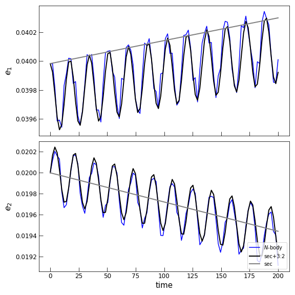
All three models show the same overall long-term eccentricity trends but the \(N\)-body model shows some short-term oscillations that comparison with the pham_full model reveals is mainly due to the effects of the 3:2 MMR. Next, we’ll capture these oscillations using a Lie series transformation.

6.2.2.2. Incorporating Lie transformations

Now we’ll redo our integration with the secular model while using the Lie transformation methods and the FirstOrderGeneratingFunction class to account for these oscillations. We’ll still be integrating our purely secular equtions of motion but the application of the Lie series transformation will allow us to approximate the effect of the 3:2 terms using a perturbative approach. We’ll construct a first-order generating function that eliminates the oscillating terms

H_3to2 = pham_full.H - pham_sec.H
H_3to2

\[\begin{split}\begin{multline} - \frac{C_{(3,-2,-1,0,0,0)}^{(0,0,0,0),(0,0)}(\alpha_{1,2}) G m_{1} m_{2} \left(\frac{\eta_{1} \sin{\left(2 \lambda_{1} - 3 \lambda_{2} \right)}}{\sqrt{\Lambda_{1,0}}} + \frac{\kappa_{1} \cos{\left(2 \lambda_{1} - 3 \lambda_{2} \right)}}{\sqrt{\Lambda_{1,0}}}\right)}{a_{2,0}} \\- \frac{C_{(3,-2,0,-1,0,0)}^{(0,0,0,0),(0,0)}(\alpha_{1,2}) G m_{1} m_{2} \left(\frac{\eta_{2} \sin{\left(2 \lambda_{1} - 3 \lambda_{2} \right)}}{\sqrt{\Lambda_{2,0}}} + \frac{\kappa_{2} \cos{\left(2 \lambda_{1} - 3 \lambda_{2} \right)}}{\sqrt{\Lambda_{2,0}}}\right)}{a_{2,0}} \end{multline}\end{split}\]

We construct our desired transformation using:

from celmech.lie_transformations import FirstOrderGeneratingFunction
pchi = FirstOrderGeneratingFunction(pham_sec.state)
pchi.add_MMR_terms(3,1)
pchi.chi

\[\begin{split}\begin{multline} - \frac{C_{(3,-2,-1,0,0,0)}^{(0,0,0,0),(0,0)}(\alpha_{1,2}) G m_{1} m_{2} \left(\frac{\eta_{1} \cos{\left(2 \lambda_{1} - 3 \lambda_{2} \right)}}{\sqrt{\Lambda_{1,0}}} - \frac{\kappa_{1} \sin{\left(2 \lambda_{1} - 3 \lambda_{2} \right)}}{\sqrt{\Lambda_{1,0}}}\right)}{a_{2,0} \left(\frac{3 G^{2} M_{2}^{2} \mu_{2}^{3}}{\Lambda_{2}^{3}} - \frac{2 G^{2} M_{1}^{2} \mu_{1}^{3}}{\Lambda_{1}^{3}}\right)} \\ - \frac{C_{(3,-2,0,-1,0,0)}^{(0,0,0,0),(0,0)}(\alpha_{1,2}) G m_{1} m_{2} \left(\frac{\eta_{2} \cos{\left(2 \lambda_{1} - 3 \lambda_{2} \right)}}{\sqrt{\Lambda_{2,0}}} - \frac{\kappa_{2} \sin{\left(2 \lambda_{1} - 3 \lambda_{2} \right)}}{\sqrt{\Lambda_{2,0}}}\right)}{a_{2,0} \left(\frac{3 G^{2} M_{2}^{2} \mu_{2}^{3}}{\Lambda_{2}^{3}} - \frac{2 G^{2} M_{1}^{2} \mu_{1}^{3}}{\Lambda_{1}^{3}}\right)} \end{multline}\end{split}\]

This is precisely the generating function that eliminates the desired terms at first order. We can even confirm the equation \([H_\mathrm{Kep},\chi] = -H_{3:2}\), where \(H_{3:2}\) are the oscillating terms associated with the 3:2 MMR, using sympy:

Hkep = PoincareHamiltonian(Poincare.from_Simulation(sim))
sp.simplify(pchi.Lie_deriv(Hkep.H) + H_3to2)

where the last line evaluates to 0. Now we do the integration:

N = 100
Tfin = 200
times = np.linspace(0,Tfin,N)
e_sec_mean,e_sec_osc = np.zeros((2,2,N))
for i,t in enumerate(times):
 # convert initial osculating values to mean ones
 pchi.osculating_to_mean()
 pham_sec.integrate(t)
 for j,p in enumerate(pham_sec.particles[1:]):
     e_sec_mean[j,i] = pham_sec.particles[j+1].e

 pchi.mean_to_osculating()
 # convert mean back to
 for j,p in enumerate(pham_sec.particles[1:]):
     e_sec_osc[j,i] = pham_sec.particles[j+1].e

The calls to osculating_to_mean() and mean_to_osculating() convert the values of of the canonical variables stored by pham_sec.state back and forth between the “primed” and “unprimed” values related by \((q',p') = \exp[\mathcal{L}_{\chi}](q,p)\) so that e_sec_mean will store “mean” values that evolve according to the Hamiltonian pham_sec.H while e_sec_osc includes oscillations due to the 3:2 MMR terms. These oscillations are computed analytically using the Lie transformation formalism. Comparing our solutions for the osculating and mean eccentricities to the results of our original integrations, we find

Now the ‘mean’ eccentricity variables track the overall trend and we’ve eliminated the initial offset of these mean values by applying osculating_to_mean before commencing the integration. The analytically-calculated correction from mean to osculating variables also match nicely with the direct integration of both the Hamiltonian, pham_full, as well as direct \(N\)-body.

The mean eccentricity trends of our simple secular model acutally begins to diverge somewhat from the integration of the fuller Hamiltonian model, suggesting a small frequency difference in the secular frequencies between the two models. This small frequency difference arises from terms that are second order in mass. Normally such terms would be negligible, but they are amplified by a small denominator in this case because the system lies near the 3:2 MMR. Second-order in mass corrections and the effect of nearby MMRs are discussed in the Section ‘Corrections to Secular Dynamics Near Resonance’.

6.2.2.3. Complete Elimination of 0th Order Terms

In the example presented above, we used a Lie series transformation to eliminate two disturbing function harmonics with frequency \(3n_2 - 2n_1\) from the Hamiltonian by adding two corresponding terms to the generating function. When adding individual terms to the generating function in this fashion, we are typically limited in the number of terms we can practically eliminate from the transformed Hamiltonian. However, it is possible with the addition of a single term to the generating function to eliminate all harmonics of the synodic frequency, \(n_\mathrm{syn} = n_1 - n_2\), to zeroth order in eccentricities and inclinations. For circular, planar orbits, the interaction Hamiltonian is

\[H_{\mathrm{int},0} = \frac{Gm_jm_i}{a_j} \left( P(\lambda_j - \lambda_i; \alpha_{ij}) -\frac{1}{\sqrt{\alpha}}\cos(\lambda_i-\lambda_j) \right)\]

where

\[P(\psi;\alpha)=\frac{1}{\sqrt{1 + \alpha^2 - 2\alpha\cos(\psi)}}~.\]

The oscillating part of this interaction term can be eliminated at first order in planet masses with the generating function

\[\chi_{0} = -\frac{Gm_im_j}{a_jn_\mathrm{syn}}\left(-\frac{1}{\sqrt{\alpha_{ij}}}\sin({\lambda_i-\lambda_j}) + \int^{\lambda_i-\lambda_j}_{0}\left(P(\psi,\alpha_{ij}) - \bar{P}(\alpha_{ij})\right) d\psi \right)~,\]

where \(\bar{P}(\alpha) = \frac{1}{2\pi}\int_{-\pi}^{\pi}P(\psi,\alpha)d\psi\) is the mean value of \(P(\psi,\alpha)\). The integral over \(\psi\) can be expressed in closed form using elliptic functions as

\[\int^{\psi}_{0}\left(P(\psi',\alpha) - \bar{P}(\alpha)\right) d\psi' = \frac{2}{1-\alpha}F\left(\frac{\psi}{2}\bigg|-\frac{4\alpha}{(1-\alpha)^2}\right) - \frac{2}{\pi}\mathbb{K}(\alpha^2)\psi\]

where \(\mathbb{K}\) and \(F\) are complete and incomplete elliptic integrals of the first kind, respectively. The term, \(\chi_0\) that eliminates all zeroth order harmonics from the interaction Hamiltonian can be added to the generating function represented by a FirstOrderGeneratingFunction instance using the add_zeroth_order_term() method.

6.3. API

class celmech.canonical_transformations.CanonicalTransformation(old_qp_vars, new_qp_vars, old_to_new_rule=None, new_to_old_rule=None, old_to_new_simplify=None, new_to_old_simplify=None, params={}, **kwargs)

A class for representing canonical transformations.

An instance represents a transformation from old canonical variables, \((q,p)\) to new variables \((q',p')\).

old_qp_vars

A list of symbols representing the old variables, \((q,p)\). The list should contain all coordinate variables, \(q\), followed by their conjugate momentum variables \(p\).

Type

list

new_qp_vars

A list of symbols representing the new variables, \((q',p')\). The list should contain all coordinate variables, \(q'\), followed by their conjugate momentum variables \(p'\).

Type

list

old_to_new_rule

A dictionary defining the substitution rules applied to transform from old canonical variables to new ones.

Type

dictionary

new_to_old_rule

A dictionary defining the substitution rules applied to transform from new canonical variables to old ones.

Type

dictionary

old_to_new_simplify

A function that will be applied to expressions when transforming from old to new variables.

Type

function

new_to_old_simplify

A function that will be applied to expression when transforming from new to old variables.

Type

function

params

A dictionary setting the numerical values of any parameters on which the transformation depends.

Type

dict

H_scale

A factor by which the transformation rescales the Hamiltonian. This is used when applying transformations that simulatneously rescale the momenta and the Hamiltonian.

Type

symbol or float

classmethod Lambdas_to_delta_Lambdas(pham)

Generate a canonical transformation applicable to a PoincareHamiltonian object, pham, that replaces the canonical momenta \(\Lambda_i\) conjugate to the mean longitudes \(\lambda_i\) with new momenta \(\delta\Lambda_i = \Lambda_i - \Lambda_{i,0}\).

N_new_to_old(exprn)

Same as new_to_old() but with numerical values replacing any symbolic parameters.

N_old_to_new(exprn)

Same as old_to_new() but with numerical values replacing any symbolic parameters.

classmethod actions_to_delta_actions(old_qp_vars, actions, delta_actions, actions_ref, params={})

Generate a canonical transformation applicable to a PoincareHamiltonian object, pham, that replaces the canonical momenta \(\Lambda_i\) conjugate to the mean longitudes \(\lambda_i\) with new momenta \(\delta\Lambda_i = \Lambda_i - \Lambda_{i,0}\).

classmethod cartesian_to_polar(old_qp_vars, indices=None, polar_symbol_pairs=None, **kwargs)

Initialize a canonical transformation that transforms a user-specified subset of conjugate coordinate-momentum pairs, \((q_i,p_i)\), to new ‘polar-style’ variable pairs

\[(Q_i,P_i) = \left(\tan^{-1}(q_i/p_i), \frac{1}{2}(q_i^2+p_i^2)\right)\]

Parameters

• old_qp_vars (array-like) – The list of old canonical variables

• indices (array-list) – List of integer indices of the coordinate-momentum pairs to be transformed.

• polar_symbol_pairs (list, optional) – List of symbols to use for the new polar-style variables. Default symbols are \((Q_i,P_i)\) where the index i ranges over the number of variable pairs being transformed.

Returns

The resulting transformation.

Return type

.CanonicalTransformation

classmethod composite(transformations, old_to_new_simplify=None, new_to_old_simplify=None)

Create a canonical transformation as the composition of canonical transformations.

Parameters

transformations (list of CanonicalTransformation) –

List of transformations to compose. Transformations are composed in the order

\[T_N \circ T_{N-1}\circ ...\circ T_1 \circ T_0\]

when passed the list \([T_0,T_1,...,]\).

Return type

.CanonicalTransformation

classmethod from_linear_angle_transformation(old_qp_vars, Tmtrx, old_cartesian_indices=[], new_cartesian_indices=[], **kwargs)

Produces the transformation \((\pmb{q},\pmb{p})\rightarrow(\pmb{Q},\pmb{P})\) given by

\[\begin{eqnarray} \pmb{Q} = T \cdot \pmb{q} ~&;~ \pmb{P} = (T^{-1})^\mathrm{T} \cdot \pmb{p} \end{eqnarray}\]

where \(T\) is a user-specified matrix.

Parameters

• old_qp_vars (list) – List of old variable symbols.

• Tmtrx (array-like) – Matrix defining the canonical transformation.

• old_cartesian_indicies (list) – List of indices specifying which old variables are cartesian-style pairs.

• new_cartesian_indicies (list) – List of indices specify which new variables should be created as cartesian style pairs.

Return type

.CanonicalTransformation

classmethod from_poincare_angles_matrix(p_vars, Tmtrx, new_qp_pairs=None, **kwargs)

Given an input Poincare instanace and an invertible matrix, \(T\), generate a transformation for which the new angle variables are given by

\[\begin{split}\pmb{Q} = T \cdot \begin{pmatrix} \lambda_1 \\ \vdots \\ \lambda_N \\ \gamma_1 \\ \vdots \\ \gamma_N \\ q_1 \\ \vdots \\ q_N \end{pmatrix}~.\end{split}\]

Parameters

• pvars (celmech.poincare.Poincare) – A Poincare instance with variables to which the resulting transformation will apply.

• Tmtrx (ndarray, shape (N,N)) – An invertible matrix determining the new canonical angle variables as linear combinations of the planets’ orbital elements.

• new_qp_pairs (list, optional) – A list of the symbols to use for the newly-generated coordinate-momentum pairs. List entries should be given in the form of 2-tuples containing a coordinate symbol followed by its conjugate momentum variable. If no list is supplied, the default symbols \((Q_i,P_i)\) will be used.

Returns

The resulting transformation.

Return type

.CanonicalTransformation

classmethod from_type2_generating_function(F2func, old_qp_vars, new_qp_vars, **kwargs)

Initialize a canonical transformation derived from a type 2 generating function. Given a set of old variables \((q,p)\), new variables, \((Q,P)\) and generating function \(F_2(q,P)\), the transformation rules are given by

\[\begin{split}p &=& \frac{\partial }{\partial q}F_2(q,P) \\ Q &=& \frac{\partial }{\partial P}F_2(q,P)\end{split}\]

Parameters

• F2func (sympy expression) – The type 2 generating function

• old_qp_vars (array-like) – The list of old canonical variables

• new_qp_vars (array-like) – The list of new canonical variables

Returns

The resulting transformation.

Return type

.CanonicalTransformation

new_to_old(exprn)

Transform an expression in terms of new canonical variables to one in terms of old varialbes.

Parameters

exprn (sympy expression) – The expression to transform.

Returns

The transformed expression.

Return type

sympy expression

new_to_old_array(arr)

Convert an array of new variable values to the corresponding values of old canonical variables.

Parameters

arr (array-like) – Value of new variables

Returns

new_arr – Array of old variable values.

Return type

numpy.array

old_to_new(exprn)

Transform an expression in terms of old canonical variables to one in terms of new varialbes.

Parameters

exprn (sympy expression) – The expression to transform

Returns

The transformed expression.

Return type

sympy expression

old_to_new_array(arr)

Convert an array of old variable values to the corresponding values of new canonical variables.

Parameters

arr (array-like) – Value of old variables

Returns

new_arr – Array of new variable values.

Return type

numpy.array

old_to_new_hamiltonian(ham, do_reduction=False)

Apply canonical transformation to a Hamiltonian object, transforming the Hamiltonian and producing a new object with a state attribute representing the phase space position in the new canonical variables.

Parameters

• ham (celmech.hamiltonian.Hamiltonian) – The Hamiltonian object to which transformation is applied.

• do_reduction (bool, optional) – If True, automatically reduce the number of degrees of freedom by detecting which canonical variables do not appear in the expression of the transformed Hamiltonian.

Returns

new_ham – The transformed Hamiltonian.

Return type

celmech.hamiltonian.Hamiltonian

classmethod polar_to_cartesian(old_qp_vars, indices=None, cartesian_symbol_pairs=None, **kwargs)

Initialize a canonical transformation that transforms a user-specified subset of conjugate coordinate-momentum pairs, \((q_i,p_i)\), to new ‘cartesian-style’ variable pairs

\[(Q_i,P_i) = \left(\sqrt{2p_i}\sin q_i,\sqrt{2p_i}\cos q_i\right)\]

Parameters

• old_qp_vars (array-like) – The list of old canonical variables

• indices (array-list) – List of integer indices of the coordinate-momentum pairs to be transformed.

• cartesian_symbol_pairs (list, optional) – List of symbols to use for the new cartesian-style variables. Default symbols are \((y_i,x_i)\) where the index i ranges over the number of variable pairs being transformed.

Returns

The resulting transformation.

Return type

.CanonicalTransformation

classmethod rescale_transformation(qp_pairs, scale, cartesian_pairs=[], **kwargs)

Get a canonical transformation that simulatneously rescales the Hamiltonian and canonical momenta by a common factor.

Parameters

• qp_pairs (list of 2-tuples) – Pairs of canonically conjugate variable symbols.

• scale (symbol or real) – Re-scaling factor. The new momenta will be given by p’ = scale * p and the new Hamiltonian will be H’ = scale * H.

• pairs (cartesian) – List of indices of Cartesian-style canonical pairs. These pairs will be recscaled such that (y’,x’) = sqrt(scale) * (y,x)

test_canonical()

Test whether the substitution rules of this tranformation constitute a canonical transformation.

Returns

Returns True if the transformation is canonical.

Return type

bool

class celmech.lie_transformations.FirstOrderGeneratingFunction(pvars)

A class representing a generating function that maps from the ‘osculating’ canonical variables of the full \(N\)-body problem to ‘mean’ variables of an ‘averaged’ Hamiltonian or normal form.

The generating function is constructed to first order in planet-star mass ratios by specifying indivdual cosine terms to be eliminated from the full Hamiltonian.

This class is a sub-class of celmech.poincare.PoincareHamiltonian and disturbing function terms to be eliminated are added in the same manner that disturbing function terms can be added to celmech.poincare.PoincareHamiltonian.

chi

Symbolic expression for the generating function.

Type

sympy expression

N_chi

Symbolic expression for the generating function with numerical values of paramteters substituted where applicable.

Type

sympy expression

state

A set of Poincare variables to which transformations are applied.

Type

celmech.poincare.Poincare

N

Number of particles

Type

int

particles

List of PoincareParticle objects making up the system.

Type

list

add_cosine_term(k_vec, max_order=None, l_max=0, nu_vecs=None, l_vecs=None, indexIn=1, indexOut=2, eccentricities=True, inclinations=True)

Add a specific cosine term to the disturbing function up to an optional max_order in the eccentricities and inclinations.

Parameters

• k_vec (Tuple of 6 ints) – Coefficients (k1, k2, k3, k4, k5, k6) for a cosine term of the form cos(k1*lambdaOut + k2*lambdaIn + k3*pomegaIn + k4*pomegaOut + k5*OmegaIn + k6*OmegaOut) Note the ks must sum to zero, and by convention we write lambdaOut first, e.g., (3, -2, -1, 0, 0, 0) is cos(3*lambdaOut - 2*lambdaIn - pomega1)

• max_order (int, optional) – Maximum order to go to in the (combined) eccentricities and inclinations. Can specify either max_order OR nu_vecs (see below), but not both (most users will use max_order). If neither are passed, max_order defaults to the leading order of the cosine term specified by k_vec.

• l_max (int, optional) – Maximum degree of expansion in \(\delta = (\Lambda-\Lambda_0)/\Lambda_0\) to include in cosine coefficients. Default is 0. Can specify either l_max OR l_vecs (see below), but not both (most users will use l_max).

• nu_vecs (List of 4-tuples, optional) – A list of the specific combinations of nu indices to include for the cosine term coefficient, e.g., [(0, 0, 0, 0), (1, 0, 0, 0), …] See paper and examples for definition and use. Can specify either max_order OR nu_vecs, but not both (max_order makes more sense for most use cases).

• l_vecs (List of 2-tuples, optional) – A list of the specific combinations of l indices to include for the cosine term coefficient, e.g., [(0, 0), (1, 0), (2, 0), …] See paper and examples for definition and use. Can specify either l_max OR l_vecs, but not both (l_max makes more sense for most use cases). One use case for passing particular l_vecs is if one body is massless, so the other Lambda doesn’t vary (and doesn’t need expansion)

• indexIn (int, optional) – Index of inner planet. Default 1.

• indexOut (int, optional) – Index of outer planet. Default 2.

• eccentricities (bool, optional) – By default, includes all eccentricity terms. Can set to False to exclude any eccentricity terms (e.g., fixed circular orbits).

• inclinations (bool, optional) – By default, includes all inclination terms. Can set to False to exclude any inclination terms (e.g., co-planar systems).

add_zeroth_order_term(indexIn=1, indexOut=2)

Add generating function term that elimiates planet-planet interactions to 0th order in inclinations and eccentricities.

The added generating function term cancels the term

\[-\frac{Gm_im_j}{a_j}\left(\frac{1}{\sqrt{1+\alpha^2-2\cos(\lambda_j-\lambda_i)}} - \frac{1}{2}b_{1/2}^{(0)}(\alpha) -\frac{\cos(\lambda_j-\lambda_i)}{\sqrt{\alpha}} \right)\]

from the Hamiltonian to first order in planet-star mass ratios.

Parameters

• indexIn (int, optional) – Index of inner planet

• indexOut (int, optional) – Index of outer planet

get_perturbative_solution(expression, free_variables=[], correction_only=False, lambdify=False, time_symbol=None)

Calculate a solution for the time evolution of an expression using first-order perturbation theory.

Parameters

• expression (sympy expression) – Expression in terms of canonical variables for which to compute a perturbative solution.

• free_variables (list, optional) – List of canonical variables to leave undetermined in the derived expression. By default, free_variables is empty and numerical values are substituted for all canonical variables

• correction_only (bool, optional) – If True, only return the perturbative correction to the expression. I.e., if expression is \(f(q,p)\) then only return \([f(q,p),\chi(q,p)]\). Otherwise, return \(f(p,q) + [f(q,p),\chi(q,p)]. Default is \).

• lambdify (bool, optional) – If True, return a function using sympy.lambdify. The list of arguments accepted by the returned function will the list free_variables, followed by the time at which to evaluate the expression.

• time_symbol (sympy.Symbol, optional) – Symbol to use for denoting time. If no symbol is given, \(t\) is used.

Returns

result – An expression for the solution as a function of time.

Return type

sympy expression or function

mean_to_osculating(**integrator_kwargs)

Convert the state’s variables from osculating to mean canonical variables.

mean_to_osculating_state_vector(y, approximate=True, **integrator_kwargs)

Convert a state vector of canonical variables of mean variables used by a normal form to un-averaged variables of the full \(N\)-body Hamiltonian.

Parameters

• y (array-like) – State vector of ‘averaged’ canonical variables.

• approximate (bool, optional) –

  If True, Lie transformation is computed approximately to first order. In other words, the approximation

  \[\exp[{\cal L}_{\chi}]f \approx f + \left[f,\chi \right]\]

  is used. Otherwise, the exact Lie transformation is computed numerically.

Returns

yosc – State vector of osculating canonical variables.

Return type

array-like

osculating_to_mean(**integrator_kwargs)

Convert the state’s variables from osculating to mean canonical variables.

osculating_to_mean_state_vector(y, approximate=True, **integrator_kwargs)

Convert a state vector of canonical variables of the the un-averaged \(N\)-body Hamiltonian to a state vector of mean variables used by a normal form.

Parameters

• y (array-like) – State vector of un-averaged variables.

• approximate (bool, optional) –

  If True, Lie transformation is computed approximately to first order. In other words, the approximation

  \[\exp[{\cal L}_{\chi}]f \approx f + \left[f,\chi \right]\]

• False (is used. If) –

• computed (the exact Lie transformation is) –

• numerically. –

Returns

ymean – State vector of transformed (averaged) variables.

Return type

array-like