5. Generic Hamiltonians¶

5.1. Introduction¶

The PoincareHamiltonian class is a special sub-class of the more general Hamiltonian class that celmech uses to model generic Hamiltonian system. We will illustrate some of the basic features of the class by using it to model the dynamics of a simple pendulum.

import numpy as np
from sympy import symbols,cos,sqrt
from celmech.hamiltonian import Hamiltonian,PhaseSpaceState
p,theta,m,g,l=symbols("p,theta,m,g,l")
H = p*p/2/(m*l*l) + (m*g*l) * (1 - cos(theta))
theta0,p0=np.pi/2,0
state = PhaseSpaceState([theta,p],[theta0,p0])
pars=dict()
pars[g]=9.8
pars[l] = 1
pars[m] = 0.15
ham = Hamiltonian(H,pars,state)
ham.H

To initialiazie a Hamiltonian one must specify a sympy symbolic representation of the Hamiltonian, a dictionary specifying the numerical values of any symbolic parameters appearing in the Hamiltonian, and a PhaseSpaceState object to represent the phase space position of the system. The final line of the code block above will display a symbolic representation of the Hamiltionan:

\[\displaystyle g l m \left(1 - \cos{\left(\theta \right)}\right) + \frac{p^{2}}{2 l^{2} m}\]

Our Hamiltonian instance also automatically generates and stores symbolic representations of the equations of motion and their Jacobian with respect to the canonical variables under the attributes flow, and jacobian:

ham.flow

\[\begin{split}\left[\begin{matrix}\frac{p}{l^{2} m}\\- g l m \sin{\left(\theta \right)}\end{matrix}\right]\end{split}\]

ham.jacobian

\[\begin{split}\left[\begin{matrix}0 & \frac{1}{l^{2} m}\\- g l m \cos{\left(\theta \right)} & 0\end{matrix}\right]\end{split}\]

After the Hamiltonian instance is initialized, it provides multiple attibutes that represent the Hamiltonian function itself, as well as the flow generated by Hamilton’s equations, and the Jacobian of those equations:

The attributes H, flow, and jacobian provide symbolic representations of the Hamiltonian, flow vector, and its Jacobian with respect to the canonical variables.
The attributes N_H, N_flow, and N_jacobian provide expressions for the Hamiltonian, flow, and Jacobian with numerical values of any parameters substituted.
The attributes H_func, N_func, and N_junc provide functions for the Hamiltonian, flow, and Jacobian that take numerical values of the canonical variables as arguments
The methods calculate_H(), calculate_flow(), and calculate_jacobian() evaluate the aforementioned functions at the current phase space position of the system, stored as the values attribue.

Hamilton’s equations of motion can be integrated using the integrate() method. When this method is called, the internal phase space state stored by the Hamiltonian under the state attribute is automatically updated. Furthermore, if any changes are made to the parameters of the Hamiltonian, the equations of motion are updated accordingly. The short integration loop below illustrates these principles:

omega0 = float(sqrt(g/l).subs(ham.H_params))
T0 = 2 * np.pi / omega0
times  = np.linspace(0,4*T0,100)
soln = np.zeros((len(times),len(ham.N_dim)))

for i,t in enumerate(times):
    # Double the length of of the pendulum at the  50th step
    if i==50:
        ham.H_params[l] *= 2
    ham.integrate(t)
    soln[i]=ham.state.values

from matplotlib import pyplot as plt
fig,ax = plt.subplots(2,1,sharex=True)
ax[0].plot(times,soln[:,0])
ax[0].set_ylabel(r"$\theta$")
ax[1].plot(times,soln[:,1],label="$p$")
ax[1].set_ylabel(r"$p$")
ax[1].set_xlabel("Time")
plt.axvline(times[50],ls='--',color='k')

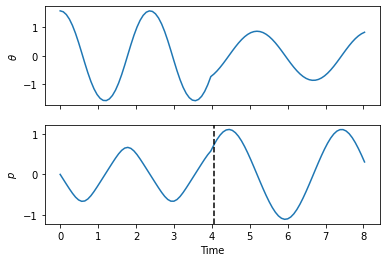
The resulting plot shows the evolution of the angle, \(\theta\), and momentum, \(p\). Note the discontinuity in the motion corresponding to when the length of the pendulum was changed in the integration loop:

5.2. API¶

class celmech.hamiltonian.Hamiltonian(H, H_params, state, full_qp_vars=None)[source]¶

A general class for describing and evolving Hamiltonian systems.

state¶

An object that stores the dynamical state of the system.

Type: object

H¶

Symbolic expression for system’s Hamiltonian.

Type: sympy expression

pqpars¶

List of canonical variable pairs.

Type: list

property H_func¶: Hamiltonian function, taking canonical variables as arguments.

Lie_deriv(exprn)[source]¶

Return the Lie derivative of an expression with respect to the Hamiltonian. In other word, compute

\[\mathcal{L}_{H}f\]

where \(f\) is the argument passed and \(\mathcal{L}_H \equiv [\cdot,H]\) is the Lie derivative operator.

Parameters: exprn (sympy expression) – The expression to take the Lie derivative of.
Returns: sympy expression for the resulting derivative.
Return type: sympy expression

N_Lie_deriv(exprn)[source]¶

Return the Lie derivative of an expression with respect to the Hamiltonian with numerical values substituted for parameters. Equivalent to N_Lie_deriv() but using the NH attribute rather than the H attribute to compute brackets.

Parameters: exprn (sympy expression) – The expression to take the Lie derivative of.
Returns: sympy expression for the resulting derivative.
Return type: sympy expression

__init__(H, H_params, state, full_qp_vars=None)[source]¶

Parameters

H (sympy expression) – Hamiltonian made up only of sympy symbols in state.qp_pairs and keys in H_params
H_params (dict) – dictionary from sympy symbols for the constant parameters in H to their value
state (PhaseSpaceState) – Object for holding the dynamical state.
above (In addition to the) –
objects (one needs to write 2 methods to map between the two) –
state_to_list(self (def) – returns a list of values from state in the same order as pqpairs e.g. [P1,Q1,P2,Q2]
state) – returns a list of values from state in the same order as pqpairs e.g. [P1,Q1,P2,Q2]
update_state_from_list(self (def) – updates state object from a list of values y for the variables in the same order as pqpairs and integrator time ‘t’
state – updates state object from a list of values y for the variables in the same order as pqpairs and integrator time ‘t’
y – updates state object from a list of values y for the variables in the same order as pqpairs and integrator time ‘t’
t) – updates state object from a list of values y for the variables in the same order as pqpairs and integrator time ‘t’

calculate_H()[source]¶

Calculate the Hamiltonian of the system in its current state.

Parameters: None –
Returns: energy – The numerical value of the Hamiltonian evaluated at the current phase space state of the system.
Return type: float

calculate_energy()¶

Calculate the Hamiltonian of the system in its current state.

Parameters: None –
Returns: energy – The numerical value of the Hamiltonian evaluated at the current phase space state of the system.
Return type: float

calculate_flow()[source]¶

Calculate the flow vector for the system in its current state.

Parameters: None –
Returns: flow – The numerical value of the flow vector evaluated at the current phase space state of the system. N is twice the number of degrees of freedom of the system.
Return type: ndarray, shape (N,)

calculate_jacobian()[source]¶

Calculate the jacobian matrix of the equations of motion for the system in its current state.

Parameters: None –
Returns: jacobian – The numerical value of the Jacobian matrix evaluated at the current phase space state of the system. N is twice the number of degrees of freedom of the system.
Return type: ndarray, shape (N,N)

property flow¶: Symbolic representation of the flow, \((\frac{\partial}{\partial p}H,-\frac{\partial}{\partial q}H)\)

property flow_func¶: Fucntion of canonical variables that returns the Hamiltonian flow vector.

integrate(time)[source]¶

Evolve Hamiltonian system from current state to input time by integrating the equations of motion.

Parameters: time (float) – Time to advance Hamiltonian system to.

property jacobian¶: Symbolic representation of the Jacobian of the flow.

property jacobian_func¶: Function of canonical variables that returns the Jacobian of the Hamiltonian flow with respect to the canonical variables.

set_integrator(name, **integrator_params)[source]¶

Set the integrator and corresponding integration parameters. This method provides a wrapper to the scipy.integrate.ode.set_integrator() method.

See here for additional details.

Parameters

name (str) – Name of the integrator.
integrator_params – Additional parameters for the integrator.

class celmech.hamiltonian.PhaseSpaceState(qp_vars, values, t=0)[source]¶

A general class for describing the phase-space state of a Hamiltonian dynamical system.

qp¶

An ordered dictionary containing the canonical coordiantes and momenta as keys and their numerical values as dictionary values.

Type: OrderedDict

qp_vars¶

List of variable symbols used for the canonical coordinates and momenta.

Type: list

qp_pairs¶

A list of the 2-tuples \((q_i,p_i)\).

Type: list

N_dof¶

The number of degrees of freedom.

Type: int

values¶

List of the numerical values of qp_vars.

Type: list

__init__(qp_vars, values, t=0)[source]¶

Parameters

qp_vars (list of symbols) – List of symbols to use for the canonical coordiantes and momenta. The list should be of length 2*N for an integer N with entries 0,…,N-1 representing the canonical coordiante variables and entries N,…,2*N-1 representing the corresponding conjugate momenta.
values (array-like) – The numerical values assigned to the canonical coordiantes and momenta.
t (float, optional) – The current time of system represented by the phase-space state. Default value is 0.

celmech.hamiltonian.reduce_hamiltonian(ham, retain_explicit=[])[source]¶

Given a Hamiltonian object, generate a new Hamiltonian object with fewer degrees of freedom by determining which (if any) canonical variables do not appear explicitly in the Hamiltonian.

Parameters

ham (Hamiltonian) – The original Hamiltonian to reduce.
retain_explicit (list) – List of variables for which to retain explicit dependence on in the transformed Hamiltonian. List entries should be either indices or variable symbols.

Returns

rham – The reduced Hamiltonian.

Return type

Hamiltonian

5. Generic Hamiltonians¶

5.1. Introduction¶

5.2. API¶

celmech

Navigation

Related Topics