7. Secular Module

7.1. Introduction

The secular module provides numerical tools to represent the secular or “orbit-averaged” dynamics of planetary systems. Secular dynamics are captured by disturbing function terms independent of the planets’ mean longitudes.

celmech provides two basic approaches to modeling a system’s secular dynamics: the first is an analytic solution to the Laplace-Lagrange system, described below in Laplace-Lagrange Solution. The second, described in Nonlinear Secular Evolution, involves numerical integration of nonlinear differential equations derived from an expansion of the equations of motion up to a user-specified maximum order in inclinations and eccentricities. Both methods can incorporate corrections to the equations of motion that are second order in planet-star mass ratios. These corrections are most important near low-order mean-motion resonances and are discussed below in Corrections to Secular Dynamics Near Resonance.

7.2. Laplace-Lagrange Solution

The classical Laplace-Lagrange solution for the secular equations of motion is derived by expressing the orbit-averaged interaction potential to leading (i.e., second-) order in eccentrictites and inclinations. At this level of approximation, the equations of motion separete into two independent sets of linear, first-order differential equations governing the eccentriticities and inclinations of the planets. These equations may be written compactly as

\[\begin{split}\frac{d}{dt}\pmb{x} = -\sqrt{-1}\pmb{S}_e \cdot \pmb{x}\\ \frac{d}{dt}\pmb{y} = -\sqrt{-1}\pmb{S}_I \cdot \pmb{y}\end{split}\]

where \(x_i = \frac{1}{\sqrt{2}}(\kappa_i - \sqrt{-1}\eta_i)\) and \(y_i = \frac{1}{\sqrt{2}}(\sigma_i - \sqrt{-1}\rho_i)\) and are derived from the ‘Laplace-Lagrange’ Hamiltonian:

\[H_\mathrm{LL} = \pmb{x} \cdot \pmb{S}_e \cdot \bar{\pmb{x}} + \pmb{y} \cdot \pmb{S}_I \cdot \bar{\pmb{y}}\]

or, in terms of orbital elements and the notation of Murray & Dermott (1999),

\[H_\mathrm{LL} = -\sum_{j=1}^{N}\sum_{i<j}\frac{Gm_im_j}{a_j}\left( f_2(e_i^2 + e_j^2) + f_{10}e_ie_j\cos(\varpi_i - \varpi_j) + f_3(s_i^2 + s_j^2) + f_{14}s_is_j\cos(\Omega_i - \Omega_j)\right)\]

The celmech.secular.LaplaceLagrangeSystem class provides utilities for computing the analytic solution to these equations of motion as well as deriving a number of properties of this solution.

A LaplaceLagrangeSystem object can be initialized directly from a Poincare object with the from_Poincare class method or from a rebound.Simulation object using the from_Simulation class method.

The example below illustrates a comparison between Laplace-Lagrange theory and N-body integration.

import numpy as np
import rebound as rb
import matplotlib.pyplot as plt
# We'll import some convenience functions for working with
# REBOUND simulations
from celmech.nbody_simulation_utilities import align_simulation, set_timestep
from celmech.nbody_simulation_utilities import get_simarchive_integration_results

# Define a function to initialize a rebound simulation.
def get_sim(scale = 0.05):
        sim = rb.Simulation()
        sim.add(m=1)
        for i in range(1,4):
            sim.add(m=i * 1e-5 , a = 2**i,
                    e = np.random.rayleigh(scale),
                    inc = np.random.rayleigh(scale),
                    l = 'uniform',
                    pomega = 'uniform',
                    Omega = 'uniform'
                   )
        sim.move_to_com()
        align_simulation(sim)

        sim.integrator = 'whfast'
        sim.ri_whfast.safe_mode=0
        set_timestep(sim,1/40) # set timestep to 1/40th of shortest orbital period
        return sim

With our set-up complete, we’ll generate LaplaceLagrangeSystem instance directly from a REBOUND simulation:

from celmech.secular import LaplaceLagrangeSystem
sim = get_sim()
llsystem = LaplaceLagrangeSystem.from_Simulation(sim)

In order to compare the Laplace-Lagrange solution to N-body, we’ll integrate the system for multiple secular timescales and get the results using the get_simarchive_integration_results utility function:

Tsec = llsystem.Tsec # Shortest secular mode period of the system
sim.automateSimulationArchive("secular_example.sa",interval=Tsec/100,deletefile=True)
sim.integrate(10 * Tsec)
sa = rb.SimulationArchive("secular_example.sa")
nbody_results = get_simarchive_integration_results(sa,coordinates='heliocentric')

secular_solution generates a secular solution as a dictionary:

llsoln = llsystem.secular_solution(nbody_results['time'])

We can now plot and compare our \(N\)-body and secular solutions

fig,ax = plt.subplots(sim.N-1,2,sharex=True,figsize=(10,6))
for i in range(sim.N-1):

    ax[i,0].plot(nbody_results['time'] / Tsec, nbody_results['e'][i],'k',label="N-body")
    ax[i,0].set_ylabel("$e_{}$".format(i+1),fontsize=16)
    ax[i,1].plot(nbody_results['time'] / Tsec, nbody_results['inc'][i],'k')
    ax[i,1].set_ylabel("$I_{}$".format(i+1),fontsize=16)

    ax[i,0].plot(llsoln['time']/ Tsec, llsoln['e'][i],'gray',label="Laplace-Lagrange")
    ax[i,1].plot(llsoln['time']/ Tsec, llsoln['inc'][i],'gray')

    ax[i,0].legend(loc='upper left')

which produces 1

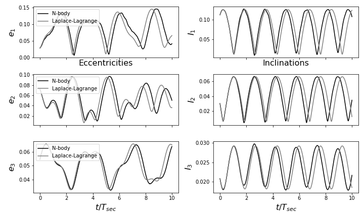
In this case, we see fair agreement between Laplace-Lagrange theory and direct \(N\)-body: the amplitudes and frequencies of eccentricity and inclination oscillations roughly agree. There are two shortcomings of the Laplace-Lagrange secular theory that can generally explain differences between analytic predictions and N-body integration results:

1. Truncating the equations of motion at leading order in inclination and eccentricity may not be sufficient

2. Period ratios near a mean motion commensurability can invalidate the secular averaging approximation

We’ll describe options for addressing both of these issues with celmech below.

7.3. Nonlinear Secular Evolution

The secular equations of motion derived from a disturbing function expansion to degree 4 or higher in eccentricity and inclination will, in general, not have analytic solutions 2. Therefore, the equations of motion need to be integrated numerically. The celmech class SecularSystemSimulation offers methods for integrating secular equations of motion derived from 4th and higher order expansions of the Hamiltonian. A SecularSystemSimulation can easily be initialized directly from a REBOUND simulation:

# grab first simulation archive snapshot
sim0=sa[0]
# intialize secular simulation object
sec_sim = SecularSystemSimulation.from_Simulation(
    sim0,
    method='RK',
    max_order = 4,
    dtFraction=1/10.,
    rk_kwargs={'rtol':1e-10,'rk_method':'GL6'}
)

Let’s briefly unpack the arguments passed to the from_Simulation call above:

• sim0 serves as the REBOUND simulation from which we’ll intialize our SecularSystemSimulation

• The method='RK' keyword argument specifies that we will integrate the equations of motion using a Runge-Kutta integrator.

• The max_order=4 keyword argument specifies that we want equations of motion derived from a 4th order expansion of the disturbing function.

• the dtFraction=1/10. tells celmech that we want to set our simulation time-step to 1/10 times the secular timescale. This secular timescale is estimated from the Laplace-Lagrange solution for the system (see llsys.Tsec above). Note that SecularSystemSimulation uses a fixed-step symplectic integration method.

• The rk_kwargs={'rtol':1e-10,'rk_method':'GL6'} argument sets the Runge-Kutta integration scheme to a 6th order Gauss-Legendre method and sets the relative tolerance of this implicit method to \(10^{-10}\). Additional integration options for SecularSystemSimulation are desrcibed in the API.

Lets run an integration with our SecularSystemSimulation and compare results to N-body. In order to do so, we’ll first define a wrapper function…

def run_secular_sim(sec_sim,times):
    N = len(times)
    # orbital elements that we want to track
    eccN,incN,pomegaN,OmegaN = np.zeros((4,sec_sim.state.N - 1,N))

    # We'll also track error in two conserved quanties,
    # the energy and the 'angular momentum deficit' or AMD
    Eerr = np.zeros(N)
    AMDerr = np.zeros(N)
    timesDone = np.zeros(N)
    E0 = sec_sim.calculate_energy()
    AMD0 = sec_sim.calculate_AMD()

    # main loop
    for i,time in enumerate(times):
        sec_sim.integrate(time)
        timesDone[i] = sec_sim.t
        E = sec_sim.calculate_energy()
        AMD = sec_sim.calculate_AMD()
        Eerr[i] = np.abs((E-E0)/E0)
        AMDerr[i] = np.abs((AMD-AMD0)/AMD0)

        # sec_sim stores a Poincare object in its 'state' attribute
        # the state is updated when the system is integrated.
        for j,p in enumerate(sec_sim.state.particles[1:]):
            eccN[j,i] = p.e
            incN[j,i] = p.inc
            pomegaN[j,i] = p.pomega
            OmegaN[j,i] = p.Omega
    return timesDone, Eerr, AMDerr, eccN, incN,pomegaN,OmegaN

… and then integrate …

T = np.linspace(0,sa[-1].t,100)
times_sec, Eerr, AMDerr, ecc_sec, inc_sec,pomega_sec,Omega_sec = run_secular_sim(sec_sim,T)

… and finally compare with our previous results:

fig,ax = plt.subplots(sim.N-1,2,sharex=True,figsize=(10,6))
for i in range(sim.N-1):
    # N-body
    ax[i,0].plot(nbody_results['time'] / Tsec, nbody_results['e'][i],'k',label="N-body")
    ax[i,0].set_ylabel("$e_{}$".format(i+1),fontsize=16)
    ax[i,1].plot(nbody_results['time'] / Tsec, nbody_results['inc'][i],'k')
    ax[i,1].set_ylabel("$I_{}$".format(i+1),fontsize=16)

    # Laplace-Lagrange
    ax[i,0].plot(llsoln['time']/ Tsec, llsoln['e'][i],'gray',label="Laplace-Lagrange")
    ax[i,1].plot(llsoln['time']/ Tsec, llsoln['inc'][i],'gray')

    # Secular Simulation
    ax[i,0].plot(times_sec/ Tsec, ecc_sec[i],'r--',label="4th Order Secular")
    ax[i,1].plot(times_sec/ Tsec, inc_sec[i],'r--')


    ax[i,0].legend(loc='upper left')

which should produce something like:

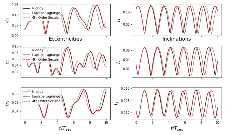
With higher-order terms in our secular equations of motion, we now have excellent agreement with \(N\)-body!

7.3.1. Integration via splitting method

In addition to direct integration of the equations of motion using Runge-Kutta schemes, the SecularSystemSimulation class offers an integration method that uses a second-order “splitting” method to solve Hamilton’s equations. This method can be selected using the method='splitting' keyword argument when initializing a SecularSystemSimulation object or by setting an object’s method attriubte to 'splitting'. (The ‘leapfrog’ and Wisdom-Holman integration methods are examples of splitting methods that may be familiar.) Our method relies on representing the Hamiltonian governing the system as the sum of two pieces:

\[\begin{split}H_\mathrm{sec} = H_\mathrm{LL} + H_\mathrm{NL} \\\end{split}\]

where \(H_\mathrm{NL}\) containts all the terms of degree 4 and higher in the components of \(\pmb{x},\bar{\pmb{x}},\pmb{y},\mathrm{ and },\bar{\pmb{y}}\).

We can, of course, solve Hamilton’s equations when the Hamiltonian is just \(H=H_\mathrm{LL}\)– this is simply the Laplace-Lagrange solution descibed above. Let’s suppose for the moment that we can also solve the equations of motion when our Hamiltonian is just \(H=H_\mathrm{NL}\). To continue, its helpful to introduce “operator notation” where \(\hat H(\tau)\) denotes the operator advancing a system for time \(\tau\) under the influence of the Hamiltonain \(H\). In other words, \(\hat H(\tau): \pmb{z}(0) \mapsto \pmb{z}(\tau)\) where \(\pmb{z}(\tau)\) is the solution to the initial value problem \(\frac{d}{dt}\pmb{z} = \Omega\cdot\nabla_{\pmb z}H(z)\) with initial data \(\pmb{z}(0)\). While we can’t solve the equations of motion for \(H_\mathrm{sec}\) exactly, we make a numerical integrator by approximating \(\hat{H_\mathrm{sec}}(\tau)\) as

\[\hat{H_\mathrm{sec}}(\tau) \approx \hat{H_\mathrm{LL}}(\tau/2)\hat{H_\mathrm{NL}}(\tau)\hat{H_\mathrm{LL}}(\tau/2) + {\cal O}(\epsilon\tau^2)\]

where \(\epsilon = |H_\mathrm{NL}|/|H_\mathrm{LL}|\sim e^2 + I^2\). In fact, by applying symplectic correctors, we can reduce the error of this integrator to \({\cal O}(\epsilon\tau^4 + \epsilon^2\tau^2)\) with relatively little computational expense. SecularSystemSimulation will apply correctors when the integrate method is called with the keywoard argument corrector=True.

There is, however, a catch to the splitting method described above: we don’t have a closed-form solution for the equations of motion generated by \({H_\mathrm{NL}}\) (if you have one we’d love to hear it!). Therefore, instead of representing the operator \(\hat{H_\mathrm{NL}}(\tau)\) exactly, SecularSystemSimulation uses an approximate solution for this evolution operator. In particular, SecularSystemSimulation solves the equations of motion generated by \(H_\mathrm{NL}\) approximately using Runge-Kutta methods. There options for exactly how SecularSystemSimulation approximates \(\hat{H_\mathrm{NL}}(\tau)\) are with the rk_kwargs argument in the same way that options for direct integration via a Runge-Kutta method are.

7.4. Corrections to Secular Dynamics Near Resonance

The secular dynamics of a multiplanet system can be significantly modified when one or more pairs of planets in the system lie near a low-order mean motion resonance. These corrections can be derived by applying canonical perturbation theory to second order in planet masses. Consider a system with a pair of planets, planets \(i\) and \(j\), near (but not in) a \(p:p-q\) MMR. A normal form Hamiltonian approximating the dynamics of the system is given by

\[\begin{split}H=H_\mathrm{Kep}(\pmb{\Lambda}) + \epsilon H_\mathrm{sec}(\pmb{z},\bar{\pmb{z}},\pmb{\Lambda}) + \epsilon H_\mathrm{res}(\pmb{z},\bar{\pmb{z}},\pmb{\Lambda},\pmb{k}\cdot\pmb{\lambda})\\\end{split}\]

where

\[H_\mathrm{res} = \sum_{n=1}^\infty e^{\mathrm{i} n \pmb{k}\cdot\pmb{\lambda} } p_n(\pmb{z},\bar{\pmb{z}},\pmb{\Lambda}) + c.c.\]

and \(\pmb{k}\cdot\pmb{\lambda} = p\lambda_{j} - (p-q)\lambda_i\). In order to derive a normal form governing the secular evolution of the system, we seek a canonical transformation that eliminates the the \(\lambda\) dependence from our Hamiltonian. In other words, we would like to find a Lie transformation such that \(H' = \exp[\epsilon{\cal L}_{\chi}] H\) is independent of \(\pmb{\lambda}\). To second order in \(\epsilon\), we have

\[\begin{split}H'= H_\mathrm{Kep}(\pmb{\Lambda}') +\epsilon\left(H_\mathrm{sec} + H_\mathrm{res} + \{H_\mathrm{Kep},\chi\}\right)\\ + \epsilon^2\left(\{H_\mathrm{sec} + H_\mathrm{res},\chi\} + \frac{1}{2}\{\{H_\mathrm{Kep},\chi\},\chi\}\right)\end{split}\]

In order to eliminate \(\pmb{\lambda}\) to first order in \(\epsilon\), we can choose

\[\chi(\pmb{z}',\bar{\pmb{z}}',\pmb{\Lambda}',\pmb{\lambda}') = \sum_{n=1}^\infty e^{\mathrm{i} n\pmb{k}\cdot\pmb{\lambda}' } \frac{p_n(\pmb{z}',\bar{\pmb{z}}',\pmb{\Lambda}')}{\mathrm{i} n\pmb{k}\cdot\pmb{\omega}(\pmb{\Lambda}')} + c.c.\]

where we have defined \(\pmb{\omega}(\pmb{\Lambda}')\equiv \nabla_{\pmb{\Lambda}'}H_\mathrm{Kep}(\pmb{\Lambda}')\). Inserting this into the expression for \(H'\), we have

\[H'= H_\mathrm{Kep}(\pmb{\Lambda}') + \epsilon H_\mathrm{sec}+ \epsilon^2\{H_\mathrm{sec},\chi\}+ \frac{\epsilon^2}{2}\{H_\mathrm{res},\chi\} + {\cal O}(\epsilon^3)\]

The terms appearing at second order in \(\epsilon\) in the expression above are a mix of oscillating terms that depend on \(\pmb{k}\cdot\pmb{\lambda}\) and secular terms that depend only on the variables \(\pmb{z}',\bar{\pmb{z}}',\pmb{\Lambda}'\). It is straightforward to show that \({\cal O}(\epsilon^2)\) secular terms arise from the term \(\frac{\epsilon^2}{2}\{H_\mathrm{res},\chi\}\). In particular, the secular terms are given by

\[ \begin{align}\begin{aligned}\begin{split}\sum_{n=1}^{\infty}\{e^{-\mathrm{i} n\pmb{k}\cdot\pmb{\lambda}'}\bar{p}_n(\pmb{z}',\bar{\pmb{z}}',\pmb{\Lambda}'), \frac{ e^{\mathrm{i} n\pmb{k}\cdot\pmb{\lambda}'} }{ \mathrm{i} n\pmb{k}\cdot\pmb{\omega}(\pmb{\Lambda}') } p_n(\pmb{z}',\bar{\pmb{z}}',\pmb{\Lambda}') \} + c.c. =\\\end{split}\\\sum_{n=1}^{\infty}\frac{1}{2} \frac{1}{\pmb{k}\cdot\pmb{\omega}(\pmb{\Lambda}')} \left({ \frac{ \pmb{k}^{\mathrm{T}} \cdot \frac{\partial\pmb{\omega}(\pmb{\Lambda}')}{\partial\pmb{\Lambda}'} \cdot \pmb{k} }{ \pmb{k}\cdot\pmb{\omega}(\pmb{\Lambda}') } p_n\bar{p}_n - \pmb{k}\cdot \frac{\partial}{\partial\pmb{\Lambda}'}(p_n\bar{p}_n) - \frac{1}{n}\left( \frac{\partial\bar{p}_n}{\partial\pmb{z}}\cdot\frac{\partial{p}_n}{\partial\bar{\pmb{z}}} - \frac{\partial{p}_n}{\partial\pmb{z}}\cdot\frac{\partial\bar{p}_n}{\partial\bar{\pmb{z}}} \right) }\right) + c.c.\end{aligned}\end{align} \]

The secular contributions of near-resonant interactions can be added to the equations of motion modeled by SecularSystemSimulation instance by using the resonances_to_include keyword argument at initialization.

7.5. API

class celmech.secular.LaplaceLagrangeSystem(G, poincareparticles=[])

A class for representing the classical Laplace-Lagrange secular solution for a planetary system.

eccentricity_matrix

The matrix \(\pmb{S}_e\) appearing in the secular equations of motion for the eccentricity variables,

\[\frac{d}{dt}(\eta_i + i\kappa_i) = [\pmb{S}_e]_{ij} (\eta_j + i\kappa_j)~.\]

or, equivalently,

\[\frac{d}{dt}\pmb{x} = -i \pmb{S}_e \cdot \pmb{x}\]

The matrix is given in symbolic form.

Type

sympy.Matrix

inclination_matrix

The matrix \(\pmb{S}_I\) appearing in the secular equations of motion for the eccentricity variables,

\[\frac{d}{dt}(\rho_i + i \sigma_i ) =[\pmb{S}_I]_{ij} (\rho_j + i \sigma_j)~.\]

or, equivalently,

\[\frac{d}{dt}\pmb{y} = -i \pmb{S}_I \cdot \pmb{y}\]

The matrix is given in symbolic form.

Type

sympy.Matrix

Neccentricity_matrix

Numerical value of the eccentricity matrix \(\pmb{S}_e\)

Type

ndarray

Ninclination_matrix

Numerical value of the inclination matrix \(\pmb{S}_I\)

Type

ndarray

Tsec

The secular timescale of the system, defined as the shortest secular period among the system’s inclination and eccentricity modes.

Type

float

eccentricity_eigenvalues

Array of the eccentricity mode eigenvalues (i.e., secular frequencies)

Type

ndarray

inclination_eigenvalues

Array of the inclination mode eigenvalues (i.e., secular frequencies)

Type

ndarray

add_first_order_resonance_term(indexIn, indexOut, jres)

Include a correction to the Laplace-Lagrange secular equations of motion that arise due to a nearby first-order mean motion resonance between two planets.

Note– corrections are not valid for planets in resonance!

Parameters

• indexIn (int) – Index of inner planet near resonance.

• indexOut (int) – Index of inner planet near resonance.

• jres (int) – Specify the jres:jres-1 mean motion resonance.

diagonalize_eccentricity()

Solve for matrix S, that diagonalizes the matrix T in the equations of motion:

\[\frac{d}{dt}(\eta + i\kappa) = i A \cdot (\eta + i\kappa)\]

The matrix S satisfies

\[T^{T} \cdot A \cdot T = D\]

where D is a diagonal matrix. The equations of motion are decoupled harmonic oscillators in the variables (P,Q) defined by

\[H + i K = S^{T} \cdot (\eta + i \kappa)\]

Returns

(T , D)

Return type

tuple of n x n numpy arrays

diagonalize_inclination()

Solve for matrix U, that diagonalizes the matrix B in the equations of motion:

\[\frac{d}{dt}(\rho + i\sigma) = i B \cdot (\rho + i\sigma)\]

The matrix S satisfies

\[U^{T} \cdot B \cdot U = D\]

where D is a diagonal matrix. The equations of motion are decoupled harmonic oscillators in the variables \((R,S)\) defined by

\[R + i S = U^{T} \cdot (\rho + i \sigma)\]

Returns

(U , D)

Return type

tuple of n x n numpy arrays

classmethod from_Poincare(pvars)

Initialize a Laplace-Lagrange system directly from a celmech.poincare.Poincare object.

Parameters

pvars (celmech.poincare.Poincare) – Instance of Poincare variables from which to initialize Laplace-Lagrange system

Returns

system

Return type

celmech.secular.LaplaceLagrangeSystem

classmethod from_Simulation(sim)

Initialize a Laplace-Lagrange system directly from a rebound.Simulation object.

Parameters

pvars (rebound.Simulation) – rebound simulation from which to initialize Laplace-Lagrange system

Returns

sim

Return type

celmech.secular.LaplaceLagrangeSystem

secular_solution(times, epoch=0)

Get the solution of the Laplace-Lagrange secular equations of motion at the user-specified times.

Parameters

• times (ndarray) – Array of times at which to evaluate the solution to the equations of motion.

• epoch (float, optional) – Current time of system state. Default is t=0.

Returns

soln – The solution dictionary contains various dynamical quantites computed at the input times.

Return type

dict

class celmech.secular.SecularSystemSimulation(state, dt=None, dtFraction=None, max_order=4, method='RK', resonances_to_include={}, rk_kwargs={})

A class for integrating the secular equations of motion governing a planetary system.

Parameters

• state (celmech.poincare.Poincare) – The initial dynamical state of the system.

• dt (float, optional) – The timestep to use for the integration. Either dt or dtFraction must be specified.

• dtFraction (float, optional) – Set the timestep to a constant fraction the period of shortest-period linear secular eigenmode.

• max_order (int, optional) – The maximum order of disturbing function terms to include in the integration. By default, the equations of motion include terms up to 4th order.

• method (str) –

  Integration method to use. Options include:

  • ’RK’ - Direct integration of equations of motion using an Runge-Kutta integration method.

  • ’splitting’ - Applies splitting to the flow generated by the system’s Hamiltonian.

• resonances_to_include (dict, optional) –

  A dictionary containing information that sets the list of MMRs for which the secular contribution will be accounted for (at second order on planet masses). Dictionary key and value pairs are specified in the form

  {(iIn,iOut) : [(j_0,k_0),...(j_N,k_N)]}
  

  include the resonances \(j_i\) : \(j_i-k_i\) with \(i=0,...,N\) between planets iIn and iOut. Note that harmonics should NOT be explicitly included. I.e., if (2,1) appears in the list [(j_0,k_0),…(j_N,k_N)] then the term (4,2) should NOT also appear; these terms’ contributions will be added automatically when the (2,1) term is added. By default, no MMRs are included.

• rk_kwargs (dict, optional) –

  Keyword arguments that determine details of the Runge-Kutta scheme used to integrate equations of motion. Keywoards include:

  • rtol: float

    Relative tolerance of root-finding step in the implicit Runge-Kutta scheme. Default is set to machine precision.

  • atol: float

    Absolute tolerance of the root-finding step in the implicit Runge-Kutta scheme. Default is 0 so that tolerance is set solely by rtol argument.

  • rk_method: str

    Runge-Kutta method to use. Available options include:

    • ’ImplicitMidpoint’

    • ’LobattoIIIB’

    • ’GL4’

    • ’GL6’

    • ’ExplicitMidpoint’

    • ’RK4’

    ’GL4’ and ‘GL6’ are Gauss-Legendre methods of order 4 and 6, respectively. ‘ImplicitMidpoint’, ‘GL4’, and ‘GL6’ are symplectic methods while ‘LobattoIIIB’ is a 4th order time-reversible method (but not symplectic). ‘ExplicitMidpoint’ and ‘RK4’ are explicit methods that are neither symplectic nor time-reversible.

  • rk_root_methodstr

    Method to use for root-finding during implicit RK step. Available options are:

    • ’Newton’

    • ’qausi-Newton’

    • ’fixed_point’

    • ’explicit’

    ’Newton’ (default) uses Newton’s method whereas ‘fixed_point’ uses a fixed point iteration method. Newton’s method requires computing the Jacobian of the equations of motion but has quadratic convergence.

property G

Value of the gravitational constant

Hamiltonian_as_polynomial(transformed=False)

Return the Hamiltonian of the secular system as a sympy.Poly object.

7. Argmunets

transformedbool, optional

If True, transform to the complex canonical variables \(\pmb{u}\) and \(\pmb{v}\), that represent the proper secular modes and are related to the usual complex canonical variables via \(\pmb{x} = T_e\cdot\pmb{u}\) and \(\pmb{y}=T_I\cdot\pmb{v}\).

returns

H – Polynomial representation of the Hamiltonian.

rtype

sympy.Poly

property Hamiltonian_coefficients_dictionary

A dictionary containing the coefficients appearing in the Hamiltonian. Dictionary is organized by pair-wise interaction terms.

property Lambda0s

Values of particle’s \(\Lambda\) canonical momenta

property N

Number of particles (including central body)

diagonalizing_tranformations()

Calculate transformations

\[\begin{split}\begin{align} D_e &=& T_e^\mathrm{T}S_e T_e\\ D_I &=& T_I^\mathrm{T}S_I T_I\\\end{split}\]

that diagonalize the matrices \(S_e\) and \(S_I\).

Returns

• Te (ndarray)

• TI (ndarray)

• De (ndarray)

• DI (ndarray)

property dt

Simulation time step

classmethod from_Simulation(sim, dt=None, dtFraction=None, max_order=4, method='RK', resonances_to_include={}, rk_kwargs={})

Initialize a SecularSystemSimulation object from a rebound simulation.

Parameters

• sim (rebound.Simulation) – REBOUND simulation to convert to SecularSystemSimulation

• dt (float, optional) – The timestep to use for the integration. Either dt or dtFraction must be specified.

• dtFraction (float, optional) – Set the timestep to a constant fraction the period of shortest-period linear secular eigenmode.

• max_order (int, optional) – The maximum order of disturbing function terms to include in the integration. By default, the equations of motion include terms up to 4th order.

• method (str) –

  Integration method to use. Options include: - ‘RK’ - Direct integration of equations of motion using an

  Runge-Kutta integration method.

  • ’splitting’ - Applies splitting to the flow generated by the system’s Hamiltonian.

• resonances_to_include (dict, optional) –

  A dictionary containing information that sets the list of MMRs for which the secular contribution will be accounted for (at second order on planet masses). Dictionary key and value pairs are specified in the form

  {(iIn,iOut) : [(j_0,k_0),...(j_N,k_N)]}
  

  include the resonances \(j_i\) : \(j_i-k_i\) with \(i=0,...,N\) between planets iIn and iOut. Note that harmonics should NOT be explicitly included. I.e., if (2,1) appears in the list [(j_0,k_0),…(j_N,k_N)] then the term (4,2) should NOT also appear; these terms’ contributions will be added automatically when the (2,1) term is added. By default, no MMRs are included.

• rk_kwargs (dict, optional) –

  Keyword arguments that determine details of the Runge-Kutta scheme used to integrate equations of motion. Keywoards include:

  • rtol: float

    Relative tolerance of root-finding step in the implicit Runge-Kutta scheme. Default is set to machine precision.

  • atol: float

    Absolute tolerance of the root-finding step in the implicit Runge-Kutta scheme. Default is 0 so that tolerance is set solely by rtol argument.

  • rk_method: str

    Runge-Kutta method to use. Available options include:

    • ’ImplicitMidpoint’

    • ’LobattoIIIB’

    • ’GL4’

    • ’GL6’

    ’GL4’ and ‘GL6’ are Gauss-Legendre methods of order 4 and 6, respectively. ‘ImplicitMidpoint’, ‘GL4’, and ‘GL6’ are symplectic methods while ‘LobattoIIIB’ is a 4th order time-reversible method (but not symplectic).

  • rk_root_methodstr

    Method to use for root-finding during implicit RK step. Available options are:

    • ’Newton’

    • ’qausi-Newton’

    • ’fixed_point’

    • ’explicit’

    ’Newton’ (default) uses Newton’s method whereas ‘fixed_point’ uses a fixed point iteration method. Newton’s method requires computing the Jacobian of the equations of motion but has quadratic convergence.

property max_order

Maximum order of disturbing function expansion in \(e\) and \(I\)

property method

Integration method to use.

Valid options are

• RK

• splitting

state_to_qp_vec()

Convert full state vector to vector of variables that enter in the secular equations.

Returns

qp_vec – Vector containing eccentricity and inclination variables \(\eta,\rho,\kappa,\sigma\). The variables are returned in the order:

\[(\eta_1,\eta_2,...,\eta_N,\rho_1,...,\rho_N,\kappa_1,...,\kappa_N,\sigma_1,...,\sigma_N)\]

Return type

ndarray

property state_vector

Current state vector of systems’ canonical Poincare variables.

property t

Simulation time

1

Since the initial conditions are randomized, results may vary

2

Only even orders of eccentricities and inclinations appear in an expansion of the secular disturbing function. Therefore, 4th order terms are the lowest nonlinear terms that appear in the secular equations.